Downloading the MIDASDB
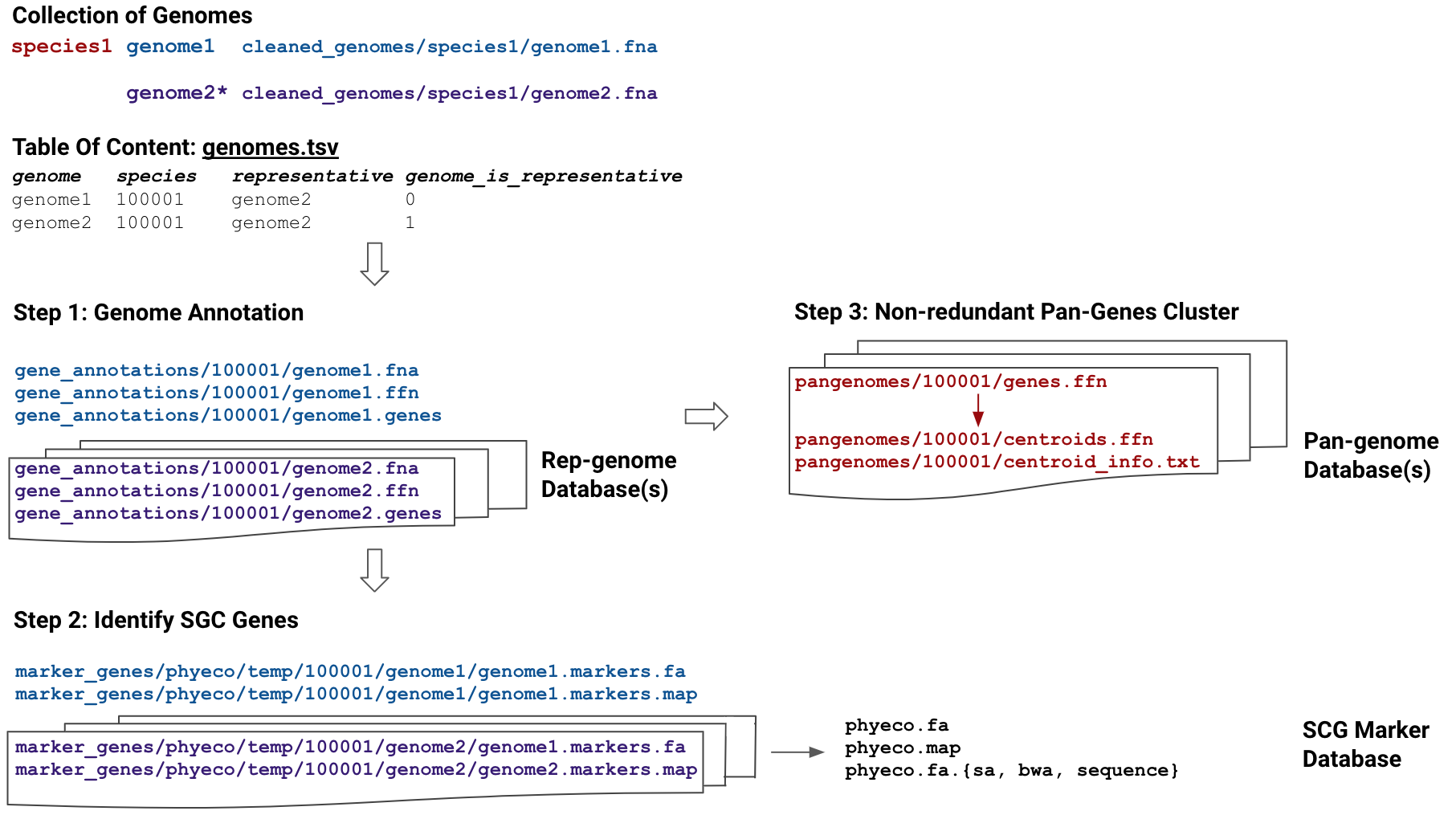
MIDAS Reference Database (MIDASDB) is comprised of three components: representative genomes,
species pangenomes, and marker genes. For each MIDASDB, six-digit numeric species ids are randomly assigned and stored in the corresponding metadata file (metadata.tsv).
For MIDAS2, we have already built two MIDASDBs from large, public, microbial genome databases:
midas2 database --list

uhgg 286997 genomes from 4644 species version 1.0
gtdb 258405 genomes from 47893 species version r202
For the purposes of this documentation we’ll generally assume that we’re working
with the prebuilt uhgg MIDASDB and that the local mirror is in a subdirectory
my_midasdb_uhgg.
Automatic database downloading is built into MIDAS2 analysis commands (e.g., run_snps and run_genes).
Specifically, MIDAS2 will download a fraction of the full
database; this subset is determined by which species are identified to be at high
coverage.
However, when parallelizing computation across samples multiple commands might try to download the same database components simultaneously, a race condition. This may be problematic.
We therefore suggest that, for large-scale analyses, users pre-download the MIDASDB.
Users should start by downloading the taxonomic marker genes.
midas2 database \
    --init \
    --midasdb_name uhgg \
    --midasdb_dir my_midasdb_uhgg
This is everything needed to run abundant species detection.
It is possible to download an entire MIDASDB using the following command:
midas2 database \
  --download \
  --midasdb_name uhgg \
  --midasdb_dir my_midasdb_uhgg \
  --species all
This requires a large amount of data transfer and storage: 93 GB for MIDASDB-uhgg
and 539 GB for MIDASDB-gtdb.
Note
The database would be much larger except that files are compressed with LZ4 to minimize storage requirements.
Alternatively, we strongly recommend that users take a more customized approach to database loading, taking advantage of species-level database sharding to download and decompress only the necessary portions of a MIDASDB.
Afterwards, we can collect a list of species present in a list of samples.
Parsing the MIDAS2 output files (midas2_output/merge/species/species_prevalence.tsv) presents a convenient way to do this.
awk '$6 > 1 {print $1}' midas2_output/merge/species/species_prevalence.tsv > all_species_list.tsv
Finally, we can download database components (both reference genomes and pangenome collections) based on these species.
midas2 database \
    --download \
    --midasdb_name uhgg \
    --midasdb_dir my_midasdb_uhgg \
    --species_list all_species_list.tsv
Afterwards, the single-sample parts of the SNV and CNV modules can be run in parallel and without a potential race condition.
Note
It is also possible for advance users to contruct their own MIDASDB from a custom genome collection (e.g. for metagenome assembled genomes).